Students explore new visualizations in Pyret, this time focusing on the frequency of observations in a quantitative dataset. They learn how to see the shape of a histogram, understand the difference between bar charts and histograms, construct histograms by hand and with Pyret, experiment with these visualizations in a contrived dataset, apply them to their own research, and interpret the results.
Students create histograms using the animals dataset
Students create visualizations of frequency using their chosen dataset, and write up their findings
Standards and Evidence Statements:
Standards with prefix BS are specific to Bootstrap; others are from the Common Core. Mouse over each standard to see its corresponding evidence statements. Our Standards Document shows which units cover each standard.
6.SP.4-5: The student summarizes and describes distributions
Data 3.1.2: Collaborate when processing information to gain insight and knowledge.
Collaboration is an important part of solving data-driven problems.
Collaboration facilitates solving computational problems by applying multiple perspectives, experiences, and skill sets.
Communication between participants working on data-driven problems gives rise to enhanced insights and knowledge.
Collaboration in developing hypotheses and questions, and in testing hypotheses and answering questions, about data helps participants gain insight and knowledge.
Collaborating face-to-face and using online collaborative tools can facilitate processing information to gain insight and knowledge.
Data 3.1.3: Explain the insight and knowledge gained from digitally processed data by using appropriate visualizations, notations, and precise language.
HSS.ID.A: Summarize, represent, and interpret data on a single count or measurement variable
S-ID.1-4: The student uses data summary techniques to aid interpretation of a single count or measurement variable
Length: 95 Minutes
Glossary:
bar chart: a visualization of categorical data in which each bar has a height corresponding to the count or proportion of values in a given category.
frequency: how often a particular value appears in a data set
histogram: A display of a quantitative variable that uses the horizontal axis to mark of regular intervals (called bins) encompassing all the values in a dataset. A bar over each bin shows the number or percent of data values in that interval, with frequency indicated in the vertical axis.
shape: The aspect of a dataset that tells which values are more or less common
Materials:
Preparation:
Computer for each student (or pair), with access to the internet
Open your Animals Starter File, and click "Run". (If you do not have this file, or if something has happened to it, you can always make a new copy.)
Let’s get some more practice working with the Design Recipe, as we prepare to do more complex analysis.
Turn to Page 22, and write the functions you see there. When you’re ready, type the contracts, purpose statements, examples and definitions into the Definitions Area.
Use the .build-column method to add a new column to the animals table, showing the weight of every animal in kilograms.
Bar Charts v. Histograms
Overview
Learning Objectives
Students review bar charts, contrasting them with histograms
Evidence Statementes
Product Outcomes
Materials
Preparation
Bar Charts v. Histograms(Time 20 minutes)
Bar Charts v. Histograms
Let’s explore two different ways of visualizing data. Complete Page 23.
Have students share their observations.
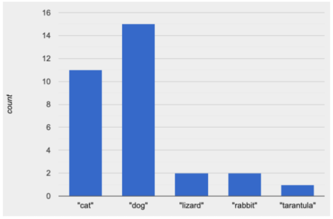
Bar charts, like the one of the bottom-left of Page 23, use the horizontal axis to show values of a categorical variable (in the diagram on the right, species). The vertical axis here shows frequency of that value in the dataset, which can be shown as absolute numbers or percentages of the total.
This bar chart happens to show the categorical values in alphabetical order from left to right, but it would be perfectly fine to re-order them any way we wish. For instance, the bar for "dogs" could have been drawn before the one for "cats". Unlike the numbers on a histogram’s horizontal axis, there is no objective order to categories on a bar-chart’s horizontal axis. For this reason, it never makes sense to talk about the "shape" of a categorical data set.
The display on the bottom-right is called a histogram. Histograms show the distribution of quantitative data. Since quantitative data can be ordered from smallest-to-largest, histograms allow us to see the shape of a data set.
Animal shelters make decisions about food, capacity and policies based on how long it takes for animals to be adopted. But looking at each value in the weeks column is tedious, and isn’t always the easiest way to make sense of the data. As the saying goes, sometimes you "can’t see the forest for the trees". Summarizing with a single number like the average alsi leaves out a lot of important information. So instead of talking about each individual in a dataset, or simply reporting the average for all those individuals, Data Scientists find it useful to describe the overall shape of the data.
A display of how long it takes animals to get adopted can make it easier to get an idea of what adoption times were most common, and if there were any unusually long or short times that it took for an animal to be adopted. Let’s take a look at a histogram of the weeks it takes an animal to be adopted. Type the following into the interactions area:
Look at the histogram and count how many animals took between 0 and 5 weeks to be adopted. How many took between 5 and 10 weeks? What else do you Notice? What do you Wonder?
Display this histogram for students to see.
What do you Notice about this histogram? What can you conclude? Here are a few conclusions to get you started:
Because we see most of the histogram’s area encompassed by the two bars between 0 and 10 weeks, we can say it was most common for an animal to be adopted in 10 weeks or less.
Because we see a small amount of the histogram’s area trailing out to unusually high values, we can say that a couple of animals took an unusually long time to be adopted: one took even more than 30 weeks.
More than half of the animals (17 out of 31) took just 5 weeks or less to be adopted. But those few unusually long adoption times pulled the average up to 5.8 weeks. Knowing about the shape gives us worthwhile information beyond the simple report of average.
If someone would ask us what was typical for the adoption times, we might say: "Almost all of the animals were adopted in 10 weeks or less, but a couple of animals took an unusually long time to be adopted - even more than 20 or 30 weeks!" Without looking at the histogram’s shape, it would have been very difficult to make this summary.
What would the histogram look like if most of the animals took more than 20 weeks to be adopted, but a couple of them were adopted in fewer than 5 weeks?
Describing Shape
Overview
Learning Objectives
Students are introduced to histograms
Evidence Statementes
Product Outcomes
Students create histograms using the animals dataset
Materials
Preparation
Describing Shape(Time 30 minutes)
Describing ShapeLet’s get some practice reading histograms, and figuring out what they mean.
Turn to Page 24, and complete the matching activity there.
Shape is one way to summarize information in a dataset, to quickly describe what values are more or less common.
A more general way to summarize the shape of a data set like this, which contains a few unusually high values, is to say that it is "skewed right, or has high outliers."
Here are the most common shapes that we see for real-world data sets:
Symmetric: values are balanced on either side of the middle.
It’s just as likely for the variable to take a value a certain distance below the middle as it is to take a value that same distance above the middle. Examples:
Heights of 12-year-olds would have a symmetric shape. It’s just as likely for a 12-year-old to be a certain number of inches below average height as it is to be that number of inches above average height.
In a standardized test, most students score fairly close to what’s average. Also, we see just as many students scoring a certain number of points above average as we see scoring that same number of points below average. The shape is symmetric (and bulges in the middle because most students score fairly close to what’s average).
Skewed left, or low outliers
Values are clumped around what’s typical, but they trail off with a few unusually low values. Examples:
Number of teeth that adults have in their mouths would be skewed left or have low outliers. Most adults will have close to a full set of 32 teeth, but a few of them with serious dental problems would have a very small number of teeth. We won’t get anyone in our data set who has 10 or 20 extra teeth in their mouths!
If most students did pretty well on an exam, but a few students performed very badly, then we’d see a shape that has left skewness and/or low outliers.
Skewed right, or high outliers
Values are clumped around what’s typical, but they trail off with a few unusually high values. We see this shape often in the real world, because there are many variables - like "income" or "time spent on the phone" - for which a few individuals have unusually high values, which aren’t balanced out by unusually low values (things like "income" and "phone time" can’t be less than zero). Examples:
Age when a woman in the U.S. gives birth would be skewed right or have high outliers. A few women would be unusually old, 40 years or even more above the average age of 26 (check the tabloids!), but none of them could be even close to 40 years below average to balance things out!
A data set of earnings almost always shows right skewness or high outliers, because there are usually a few values that are so far above average, they can’t be balanced out by any values that are so far below average. (Earnings can’t be negative.)
To build a histogram, we start by sorting all of the numbers in our column from smallest to largest, marking our x-axis from the smallest value to the largest value and dividing into equally-sized intervals, or "bins". Once we have our bins, we put each value in our dataset into the bin it belongs, and then count how many values are in each bin. This count determines the height of the bars on our y-axis.
Turn to Page 25, and try drawing a histogram from a dataset.
Note that interals on this display include the left endpoint but not the right. If we included the right endpoint and someone had 0 teeth, we’d have to add on a bar from -5 to 0, which would be awfully strange!
The size of the bins matters a lot! Bins that are too small will hide the shape of the data by breaking it into too many short columns. Bins that are too large will hide the shape by squeezing the data into just a few tall columns. In this workbook exercise, the bins were provided for you. But how do you choose a good bin-size?
Rule of thumb: a histogram should have between 5-10 bins.
Let’s make a histogram for the pounds column in the animals table, sorting the animals into 20-pound bins: histogram(animals-table, "pounds", 20)
Would you describe the shape of your histogram as being skewed left/low outliers or symmetric or skewed right/high outliers? Which one of these statements is justified by the histogram’s shape?
A few of the animals were unusually light.
A few of the animals were unusually heavy.
It was just as likely for an animal to be a certain amount below average weight as it was for an animal to be that amount above average weight.
Try bins of 1-pound intervals, then 100-pound intervals. Which of these three histograms best satisfies our rule of thumb?
Challenge: Compare histograms for pounds of cats vs. dogs in the dataset. Are their shapes different? If so, how?
On Page 26, describe the pounds histogram and another one you make yourself. When writing down what you notice, try to use the language Data Scientists use, and discuss skew and outliers.
Your Dataset
Overview
Learning Objectives
Evidence Statementes
Product Outcomes
Students create visualizations of frequency using their chosen dataset, and write up their findings
Materials
Preparation
Your Dataset(Time 20 minutes)
Your Dataset
How is your dataset distributed? Choose two quantitative variables and display them with histograms. Explain what you learn by looking at these displays. If you’re looking at a particular subset of the data, make sure you write that up in your findings on Page 27.
Give students 10-15min to make their next set, and have them share back. Encourage students to read their observations aloud, to make sure they get practice saying and hearing these observations.
Closing
Overview
Learning Objectives
Evidence Statementes
Product Outcomes
Materials
Preparation
Closing(Time 5 minutes)
ClosingHistograms are a powerful way to display a data set and assess its shape. But shape is just one of three key aspects that tell us what’s going on with a quantitative data set. In the next unit, we’ll explore the other two: center and spread.
Bootstrap:Data Science by Emmanuel Schanzer, Nancy Pfenning, Emma Youndtsmith, Jennifer Poole, Shriram Krishnamurthi, Joe Politz and Ben Lerner was developed partly through support of the National Science Foundation, (awards 1535276, 1647486, and 1738598), and is licensed under a Creative Commons 4.0 Unported License. Based on a work at www.BootstrapWorld.org. Permissions beyond the scope of this license may be available by contacting schanzer@BootstrapWorld.org.

 What do you Notice about this histogram? What can you conclude? Here are a few conclusions to get you started:
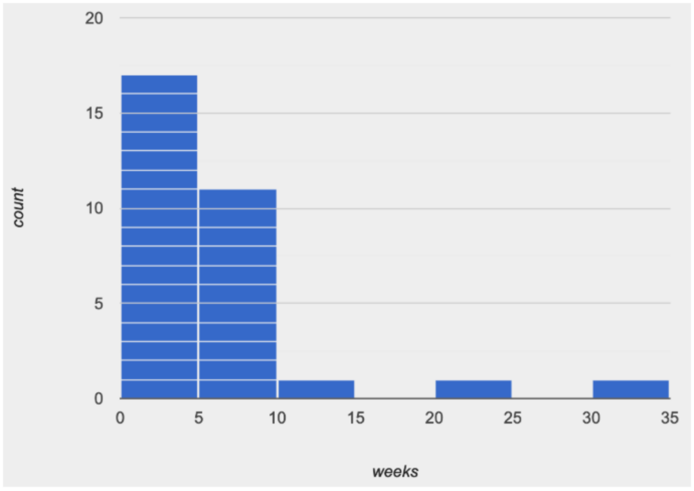 A more general way to summarize the shape of a data set like this, which contains a few unusually high values, is to say that it is