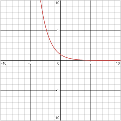
Students are introduced to exponential sequences and the parts of an exponential graph. They use our Desmos slider activity to explore how the values in the vertex form describe the shape of the model, and then talk about exponential growth and decay.
Lesson Goals |
Students will be able to…
|
Student-facing Lesson Goals |
|
Materials |
|
Preparation |
|
🔗Exponential Sequences
Overview
Having identified that the Covid scatter plot appears neither linear nor quadratic, students learn about characteristics of exponential functions in tabular form.
Launch
Let’s review what we know about the behavior of the models we’ve seen so far:
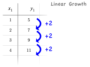 Remember that linear functions grow by fixed intervals, so the growth is constant. In the table shown here, each time the x-value increases by 1, we see that the y-value increases by 2. This is true for any set of equal-sized intervals: a line needs to slope up or down at a constant rate in order to be a straight line!
If the growth is constant, the relationship is linear.
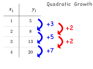 Quadratic functions grow by intervals that increase by fixed amounts! In the table to the right, the blue arrows show a differently-sized jump between identical intervals, meaning the function is definitely not linear! However, if we take a look at the difference between those differences(shown in red), we’re back to constant growth!
If the "growth of the growth" is constant, the relationship is quadratic.
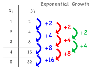 When we find the growth between the y-values, we can immediately tell it’s not linear. When we try to calculate the "growth of the growth", we see that it’s not quadratic either.
Exponential functions grow even faster than quadratics!
If we calculate the "growth of the growth of the growth" (shown in green)… we still haven’t found a constant… but we should notice that each of these "growths" just repeats the original pattern of y-values! We could calculate the third difference, fourth difference, and so on…and never reach a stopping point.
Exponential functions grow so rapidly that asking "what is being added to y?" isn’t helpful at all.
Investigate
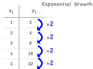
In order to talk about the growth of an exponential function we need to identify the base (or growth factor) by asking ourselves "what is being multiplied by y?"
In this case, we can see that the y-values are doubling each time, so the base / growth factor is 2!
-
Turn to What Kind of Model? (Tables), and decide what kind of pattern is represented in each table.
-
For each table that is growing exponentially, identify the base / growth factor.
Synthesize

-
What strategies did you use to decide which tables showed exponential growth v. linear or quadratic?
-
Answers will vary — but encourage students who struggled to draw the first and second differences. Everyone has at least one strategy!
-
Which table was the easiest to identify?
-
Probably table 2 — whose y-values clearly grow by a factor of 10 each time
🔗Exponential Graphs
Overview
Students learn about characteristics of exponential functions in both graphical and function notation form.
Launch
Most textbooks teach that exponential models have the form: f(x) = a(b)x + k
That’s because most textbooks only present exponential functions with a horizontal shift of zero… and when h = 0, we can safely remove it and use the simplified form of the equation.
But, just as with other models we have explored, exponential models can have a horizontal shift.
The expanded form for exponential models includes h and looks like this: f(x) = a(b)(x−h) + k
Advance your teacher dashboard of Modeling Covid Spread (Desmos) to the Slide 2: How does h transform exponential functions? and give your students time to reinforce their understanding of h−values from other models by connecting it to exponential functions.
Investigate
Let’s explore how each model setting in f(x) = a(b)x + k influences the shape of the model!
Make sure you’ve advanced your teacher dashboard of Modeling Covid Spread (Desmos) to the third slide ("Exploring Exponential Functions") so that students are looking at the correct screen.
Decide whether you want to debrief this activity with your class after each section or at the end.
-
Let’s return to the Modeling Covid Spread Desmos file.
-
You should now be on the third slide: Exploring Exponential Functions.
-
Use it to complete Graphing Exponential Models: f(x) = a(b)x + k.
-
Was it easy to guess what any of the model settings did, before you graphed them?
-
Answers will vary, but the vertical shift of k was likely the easiest one.
-
Did the behavior of any of the model settings surprise you?
-
Answers will vary, but b is likely to stand out to students.
Base b
The base of an exponential function (b) must always be positive, because exponential functions grow and decay uniformly.
A negative b would bounce from one side of the y-axis to another.
More importantly, when raised to a fractional exponent like 1/2 negative values of b might also lead to things like $$\displaystyle \sqrt{-2}$$!
| Exponential Growth | Flat | Exponential Decay |
|---|---|---|
|
|
|
b > 1
|
b = 1
|
0 < b < 1
|
Asymptotes for Exponential Functions (k)
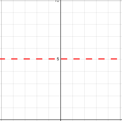
All exponential functions have an asymptote: a horizontal line at y = k that they get closer and closer to touching, but never actually reach.
Adjusting k shifts the asymptote up and down, dragging the rest of the exponential curve that approaches it.
Initial Value a
What do you think the asymptote for the exponential function below will be?
f(x) = 4(2x ) + 3
If exponential functions worked like linear functions, we might expect the y-intercept to be the the constant term: 3.
But, since any value raised to the power of zero is 1, when x = 0 in exponential equations, the a part of the exponential term remains, so we can’t just look at the constant term.
f(0) = 4(20 ) + 3
= 4(1) + 3
= 7
-
So what is the y-intercept of an exponential function?
-
Give students time to discuss…
The y-intercept of an exponential function is a + k
-
If k = 0…
-
people often "leave it out" of the function
-
the y-intercept is just a
-
-
If x = 0…
-
The y-intercept of linear models is the vertical shift
-
The y-intercept of quadratic models is the vertical shift
-
The y-intercept of exponential models is a!
-
-
Turn to What Kind of Model? (Graphs & Scatter Plots), and decide whether the shape of the scatter plot suggests a linear, quadratic, or exponential relationship.
Synthesize
-
How does finding the y-intercept for exponential functions differ from finding it for the linear and quadratic functions you’ve seen before?
-
When x is zero for linear and quadratic functions, we can ignore everything except the constant term. In exponential functions, the constant term isn’t enough to give us the y-intercept!
-
What new information have you gained by looking at graphical representations, rather than tables?
-
In the graph you can easily see the asymptote — where the function "levels out" — which is harder to see staring at number in a table.
🔗Exponential Growth and Decay
Overview
Having explored the behavior of exponential functions as sequences of numbers and point clusters on a graph, students move on to sense-making. They explore the relationship between growth/decay rates and growth/decay factors. Finally, they apply this knowledge to identifying exponential growth and decay in function definitions and word problems.
Launch
-
Complete questions 1-4, using Pyret, Desmos, or a calculator.
-
If a new car sells for $32,000, and the resale value drops by one-eighth (12.5%) each year.
-
How much is the car worth after 1 year?
-
How much is the car worth after 2 years?
-
How much is the car worth after 3 years?
-
-
Solutions:
-
1 year: $28,000
-
2 years: $24,500
-
3 years: $21,437.50
-
The less the car costs, the less "an eighth of it" costs. The car’s highest value is in the first year, so the biggest price drop happens that year as well. As the years go by and the car’s value drops, price will drop more and more slowly.
In fact, no matter how many years go by, the cost will never actually reach zero! It will just keep getting closer to zero by smaller and smaller amounts.
Let’s write a function to model this change, so that we can calculate the car’s value for each year without having to calculate the value for every year in between!
-
We know the initial value a is $32,000.
-
With the car’s value dropping, we know that the base b must be less than one. But how do we compute the base exactly?
Let’s look at the math:
-
To find the value after one year, we’d subtract $32,000 minus an eighth of $32,000.
-
$32,000 − ($32,000 × 0.125)
Factoring out $32,000 we get:
-
$32,000 × (1 − 0.125) or
-
$32,000 × (0.875)
With the value dropping by a decay rate (r) of 12.5%, we have a decay factor (b) of 87.5% (0.875).
Our function is: f(x) = 32,000 × 0.875x
In the scenario we just modeled, the value was dropping, so our function described exponential decay. To model scenarios where values rise, we use functions describing exponential growth.
When the value is dropping, the decay factor (b) will be: b = 1 − r
When the value is rising, the growth factor (b) will be: b = 1 + r
Consider a savings account that starts at $100 and grows by 3% (0.03) each year:
-
The initial value (a) is 100.
-
The growth rate (r) is 0.03, so the growth factor (b) is 1.03.
-
Our function is f(x) = 100 × 1.03x
Investigate
Exponential growth and exponential decay show up all the time!
-
Most cells (e.g. bacteria, the cells in a growing fetus, etc.) divide every few hours, doubling the number of cells each time. A single cell will split into 2, those 2 cells will split to become 4, then 8, then 16, etc: the function cells(hours) grows exponentially.
-
Unstable atomic nucleus decay into stable nuclei over time, emitting ionizing radiation as a byproduct. We use the term half-life to refer to the length of time it takes for 50% of the atomic nuclei in a radioactive sample to decay: the function unstable−atoms(half−lives) decays exponentially.
-
Car loans, savings accounts, mortgages, and credit card debt all use exponential growth (if you’re saving) and decay (if you’re borrowing). Many adults don’t really understand exponential behavior well, and don’t realize how sharply these functions rise or fall once they hit the sharp part of the curve!
In the following activities, students will:
-
identify whether various plots, scenarios, and definitions represent linear, quadratic, or exponential functions
-
think about and apply their knowledge of growth, decay, initial value, and growth factor
Decide whether you’d like to pull your class back together to discuss after each activity or once they’ve completed all three.
Let’s practice identifying linear, quadratic, and exponential growth.
-
With your partner, complete What Kind of Model? (Descriptions) and What Kind of Model? (Descriptions 2).
-
When you’re done, complete What Kind of Model? (Definitions)
-
What strategies did you use to decide if a function was linear, quadratic, or exponential?
-
When a function was exponential, how did you recognize whether it was growing or decaying?
-
What new insights did you gain about exponential functions by thinking about them in real-world scenarios?
Have students share their answers, asking them to notice and wonder about the sequences for the exponential examples. How are these sequences growing or decaying? How is that growth or decay different from what they’ve seen before?
Synthesize
-
You looked at several different representations of exponential functions: tables, graphs, descriptions, and equations.
-
Which representation was the most useful for you? Why?
-
Which representation was the least useful for you? Why?
Optional Activity: Guess the Model!
-
Divide students into small groups (2-4), and have each team come up with an exponential, real-world scenario, then have them write down an exponential function that fits this scenario on a sticky note. Make sure no one else can see the function!
-
On the board or some flip-chart paper, have each team draw a scatter plot for which their exponential function is best fit. They should only draw the point cloud — not the function itself! Finally, students title their scatter plot to describe their real-world scenario (e.g. "money in a savings account vs. years").
-
Have teams rotate so that each team is in front of another team’s scatter plot. Have them figure out the original function, write their best guess on a sticky note, and stick it next to the plot.
-
Have teams return to their original scatter plot, and look at the model their colleagues guessed. How close were they? What strategies did the class use to figure out the model?
-
The model settings can be constrained to make the activity easier or harder. For example, limiting these model settings to whole numbers, positive numbers, etc.
-
To extend the activity, have the teams continue rotating so that each group adds their sticky note for the best-guess model. Then do a gallery walk so that students can reflect: were the models all pretty close? All over the place? Were the guesses for one model setting grouped more tightly than the guesses for another?
-
🔗Additional Practice
These materials were developed partly through support of the National Science Foundation, (awards 1042210, 1535276, 1648684, 1738598, 2031479, and 1501927).  Bootstrap by the Bootstrap Community is licensed under a Creative Commons 4.0 Unported License. This license does not grant permission to run training or professional development. Offering training or professional development with materials substantially derived from Bootstrap must be approved in writing by a Bootstrap Director. Permissions beyond the scope of this license, such as to run training, may be available by contacting contact@BootstrapWorld.org.


