Students use linear models to investigate the relationship between college enrollment and median income in demographic data about US states.
Lesson Goals |
Students will be able to…
|
Student-facing Lesson Goals |
|
Materials |
|
Supplemental Materials |
|
Preparation |
|
🔗Optional Review: Defining a Line from Two Points
Overview
In the next section of this lesson, students are asked to write the Slope-Intercept form of the line, given two points in our states dataset. To prep them for success, this section is an opportunity for students to review what they already know about linear functions and the process of finding the equation of a line from a table and then practice writing linear functions, given two points on the line.
Launch
Before we learn to fit linear models to scatter plots, let’s review. What do you remember about linear functions?
We’d expect students to be able to surface much of the following:
-
Linear functions look like straight lines.
-
Vertical lines are not functions, because their slope is undefined as a result of their horizontal change being zero.
-
The steepness of a line can be described by its slope (or constant rate of change).
-
The slope can be calculated from any two points.
-
Students may remember the slope as $$\displaystyle \frac{change \; in \; y}{change \; in \; x}$$ or $$\displaystyle {rise}\over\displaystyle{run}$$ or $$\displaystyle \frac{y_2 - y_1}{x_2 - x_1}$$.
-
The point where the line crosses the y-axis is called the y-intercept or vertical shift.
-
The x-coordinate of the y-intercept always starts with zero, e.g. (0, y).
-
Diagonal lines have both a y-intercept and an x-intercept.
-
Horizontal lines have a constant rate of change of zero.
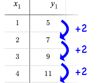
Linear relationships grow by fixed amounts, meaning that the difference between two y-values will always be the same over identical horizontal intervals. In the table shown to the right, you can see arrows pointing out the "jumps" between y-values for x-intervals of 1. Each jump is the same size: +2. |
|
If the rate of change is constant, the relationship is linear.
-
Try comparing intervals of 2, instead of intervals of 1.
-
Is the difference between y-values from x = 1 to x = 3 the same as the difference between y-values from x = 2 to x = 4?
-
Yes. When x increases by 2, y increases by 4.
-
What is the y-value when x = 0?
-
By following the pattern of the blue arrows backwards, we can subtract 2 and arrive at y = 3
-
What is the slope of this line?
-
2. It’s another word for the rate of change. The arrows show that y increases by 2 as x increases by 1.
-
What equation would describe the linear relationship we observe in this table?
-
Knowing the y-intercept and the "size of the growth", we can tell that the equation of this line is f(x) = 2x + 3.
Synthesize
-
Given two points from a line, what steps are involved in writing the slope-intercept form of the line?
-
Compute the slope.
-
Substitute the slope and the coordinates of the point into y = mx + b and compute the y-intercept.
-
Write the point-slope form of the line using the slope and y-intercept we computed.
🔗The Alaska-Alabama Model
Overview
Building on prior knowledge of linear functions, students learn to find the line of best fit to model the relationship in a scatter plot that looks linear.
Launch
-
Return to Pyret, open your copy of the State Demographics Starter File and click "Run".
-
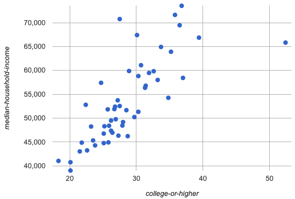
Make a scatter plot showing the relationship between
pct-college-or-higherandmedian-income, usingstatefor the labels.

-
What do you notice about the shape of this scatter plot? What pattern do you see?
-
This scatter plot appears to show a positive, linear relationship:
States with higher percentages of college graduates tend to have higher median household incomes.
 As students make predictions in response to the questions below, let them discuss and explain their thinking.
-
If possible, mark off a single point for each of the hypothetical percentages, then connect those points to show a straight line.
-
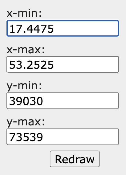
Note that some of these new points would require changing the x-min, x-max, y-min and/or y-max of our scatter plot, which we can do by typing in the cells on the right side of the scatter plot and clicking "Redraw".
Suppose the United States were to add a new state.
Based on the data for the existing 50 states (plus DC!)…
-
What median household income would you predict, if exactly 30% of the new state’s citizens had attended college?
-
Answers will vary. But should be above 50,000 and below 60,000
-
What would you predict if 20% had attended college?
-
Answers will vary. But should be around 40,000
-
If 40% had attended college?
-
Answers will vary. But should be upwards of 65,000
When we see patterns in data, we can use those patterns to make predictions.
Investigate
We can draw a line to model all the possible predictions at once and then we can write a function to describe it!
In this case, we’re looking for a model of the relationship between college graduation and income.
median−income(pct−college) = mslope × pct−college + by-intercept |
In the function above, we know that pct-college is our explanatory variable. The slope and y-intercept are model settings: numbers that specify the shape of our linear model.
We want to know: Are there model settings for m and b that will fit the data well?
We have a scaffolded version of Build a Model from Samples: College Degrees v. Income that you can share with students instead of the one in the directions below if your students need more support with finding the equation from two points.
-
If we have two points, we know how to write the point-slope form of the line. Let’s find the model that passes through our first two points: Alabama and Alaska!
-
Complete the first section of Build a Model from Samples: College Degrees v. Income.
Confirm that students were able to successfully compute the slope and y-intercept, define and test al-ak(x) in Pyret, and find how well al-ak(x) predicted several states' median income given the percentage of the population with at least a college degree.
-
Why wasn’t the Alaska-Alabama model a good fit for the rest of the data?
-
Because Alaska is an outlier that falls pretty far above the line of best fit.
-
Can you identify two other states we could have built a better model from?
-
Record your thinking on the last section of Build a Model from Samples: College Degrees v. Income. You’ll want to remember them for later!
Synthesize
-
Why do people build models for datasets?
-
So they can make predictions using the patterns they see.
-
What advice do you have for someone looking to build a model for a dataset?
-
Pick 2 points that feel representative of the trend.
🔗Optional: Horizontal Shift in Linear Functions
Overview
This section lays the ground work for exploring horizontal shift in nonlinear models by giving students a chance to explore horizontal shift in linear models (likely more intuitive more familiar and intuitive for students) using our custom Desmos slider activity.
Launch
The Slope-Intercept form of the line we’ve been using tells us about the slope (m) and the vertical shift. It is also possible to shift a line or curve horizontally, and for some of the non-linear models we will be exploring in this course, identifying the horizontal shift will be important.
To prepare ourselves for that thinking, let’s look at how horizontal shifts would fit into our linear model.
f(x) = m(x−h) + k is the expanded slope-intercept form, which allows us to change both the horizontal (h) and vertical shift (k).
Note: When the horizontal shift is zero, we can safely remove (h) from the equation. That’s exactly what we’ve been doing with our Slope-Intercept form.
Why are we using k instead of b?
Using b for the y-intercept in the point-slope form is a convention people have agreed upon over time… but the convention doesn’t hold for non-linear models.
We’re introducing h and k here to help students make the connection between the exploration they will be doing with this linear form and the nonlinear forms they will be seeing in future lessons.
Investigate
Make sure you have created a link or code for your class to Exploring Horizontal Shift in Linear Functions (Desmos).
Let’s take a moment to explore how horizontal shifts work with linear functions.
-
Open Exploring Horizontal Shift in Linear Models (Desmos).
-
Use the slider activities to complete Exploring Horizontal Shift in Linear Models.
-
Were you able to find any instances where the transformation from a horizontal shift couldn’t be achieved by a vertical shift instead?
-
No. Because lines go on forever without changing direction, horizontal shifts can always be accounted for with vertical shifts. We can prove this to ourselves algebraically because if we distribute the m in the equation f(x) = m(x−h) + k, we get f(x) = mx − mh + k and since mh and k will always be numbers, we can just add them together to get the y-intercept.
Synthesize
-
Why do math books generally not discuss horizontal shifts for linear models?
-
Because they can all be achieved through a vertical shift instead
These materials were developed partly through support of the National Science Foundation, (awards 1042210, 1535276, 1648684, 1738598, 2031479, and 1501927).  Bootstrap by the Bootstrap Community is licensed under a Creative Commons 4.0 Unported License. This license does not grant permission to run training or professional development. Offering training or professional development with materials substantially derived from Bootstrap must be approved in writing by a Bootstrap Director. Permissions beyond the scope of this license, such as to run training, may be available by contacting contact@BootstrapWorld.org.

